Master Thesis

This master thesis explores ways to apply geometric deep learning to the field of numerical simulations with an emphasis on the Navier-Stokes equations. With the recent success of Deep Learning, there should be room for experimentation also in the field of fluid simulations. Here we lead such an experiment. We propose an end-to-end differentiable architecture that allow object-to-mesh predictions of fluid simulations. We provide a comparison with a baseline and visual results on three different datasets: airfoils, backward-facing steps and winged-drones.

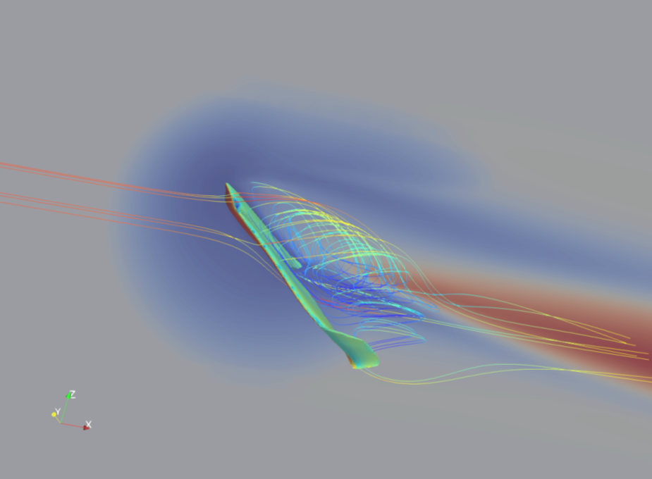
Here such a model has been built, leveraging geometric deep learning, i.e. deep learning on irregular domains, on which standard convolutions would fail. As a proof-of-concept we will present here only the results around the backward-facing-step. The interested reader is invited to visit the thesis itself for more details and different setups.

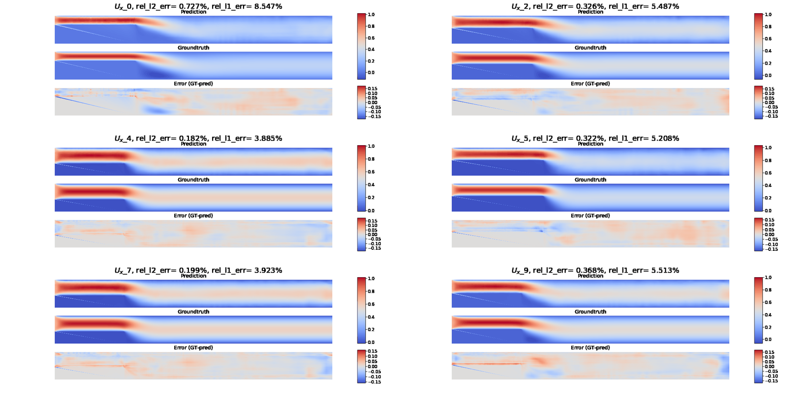
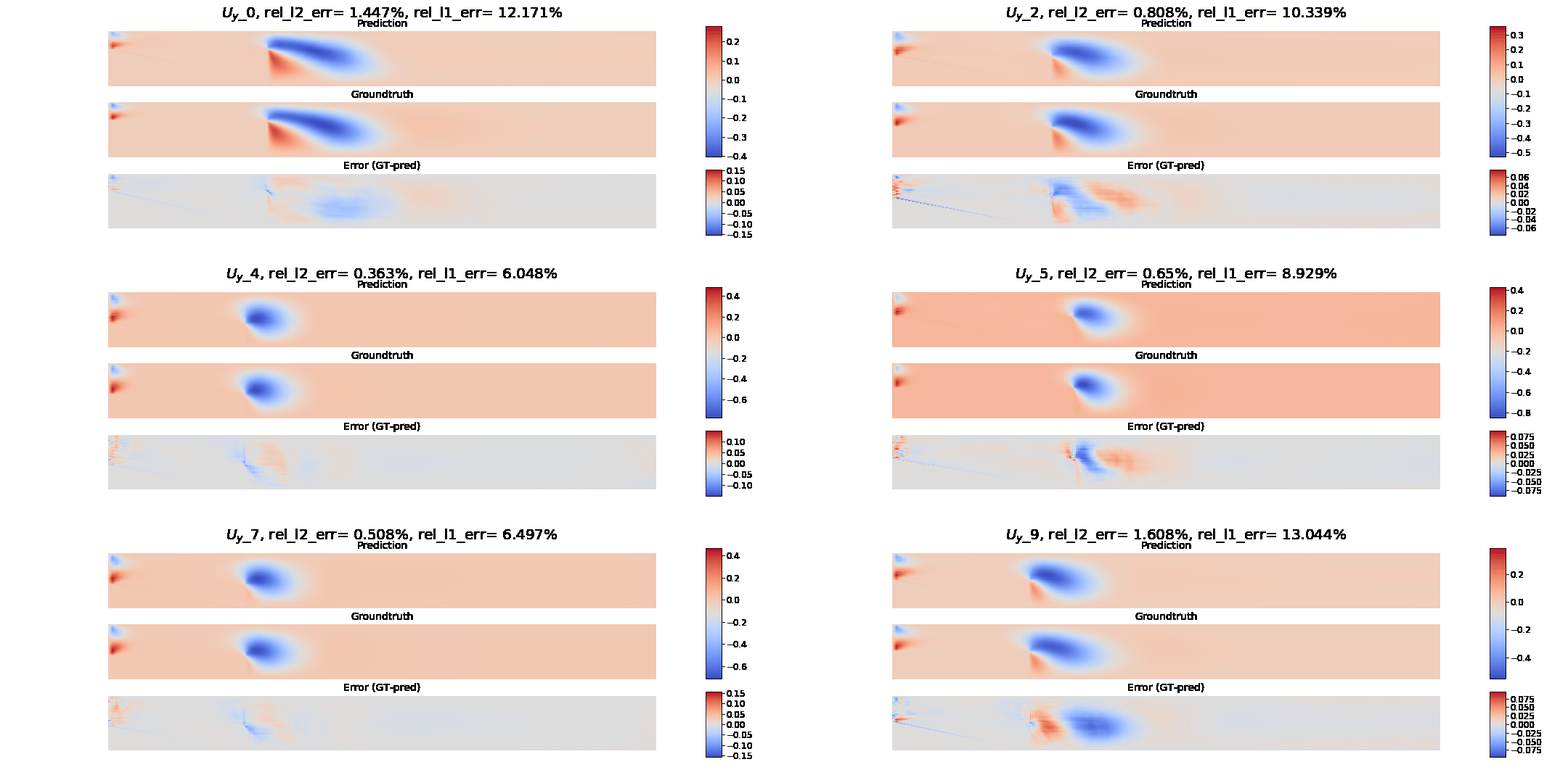
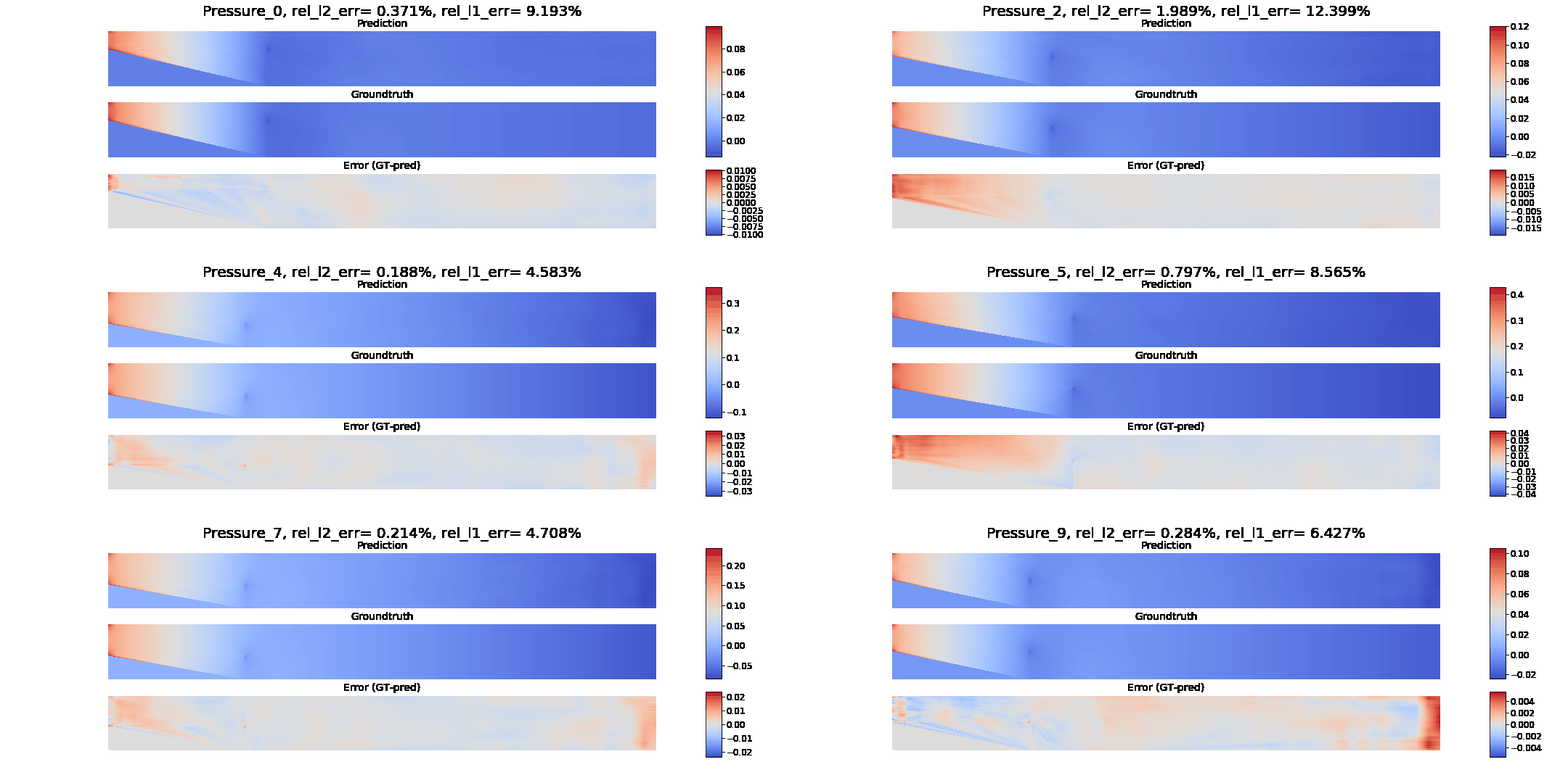
The backward facing step is an important milestone in showing result in computational fluid dynamics as it has a simple geometry that hides a complex phenomena: the recirculation zone [see next paragraph]. Our model is able to predict the internal flow around the backward-facing-step as visually shown here below, with first prediction, the groundtruth and finally the absolute point-wise error. We emphatise that the prediction was made mesh-to-mesh, with as additional information the boundary conditions and properties of the flow (e.g. viscosity).

x-Velocity:

y-Velocity:

Pressure:

Once we got all x-velocity and y-velocity we wan also predict the recirculation zone behind the step, as we illustrate below. In the figure we show the simulation [left], and prediction [right].

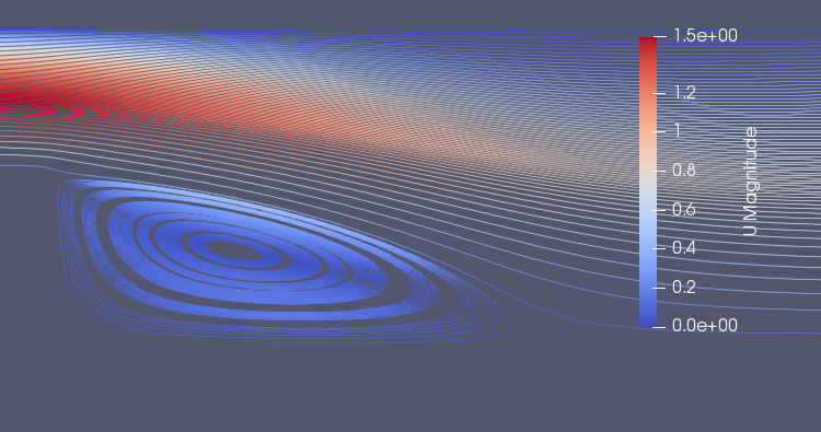
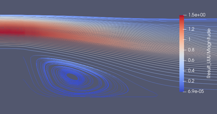
As we see, the predicted solution (right) seems unfeasible with some streamlines seemingly exiting the side of the step... And indeed it is infeasible! This is because the conservation of mass has not been enforced by the model. To correct this behaviour, we can add a penalisation term in the loss of the network or iterate one through the domain to correct the conservation.

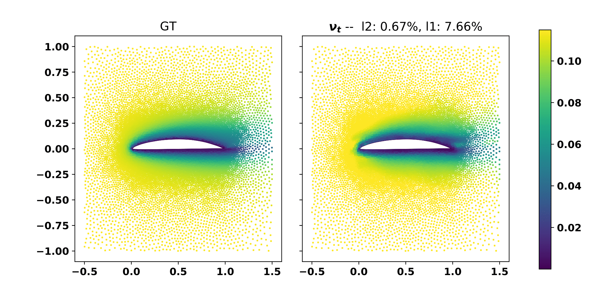
Of course, the same process can be repeated to other other fields that can be and other problems. Here below, we can see the turbulent viscosity on the airfoil dataset:

Application of such an application can range computer graphics to the automatic design of engineering shapes. However, one application that we is dear to me would be to combine this prediction to the more accurate numerical simulation. An example is to initialize an iterative solver with a corrected prediction, hence (hopefully) drastically decreasing the number of iterations necessary to reach convergence.

I hope to have captivated your attention and convinced you that there is something here that could be used in the future.
Thesis available at: infoscience